As with many mathematical problems, it is possible to define problems “dual” to an LP problem in various forms. Study of this aspect of LP problems, besides revealing interesting structural properties, has many implications and applications. This is a continuation of the siplex algorithm discussion and here is the PDF.
1.1. Primal-dual formulation and its basic properties
The primal-dual relationship for LP in general form is defined as

If we view the standard LP as a special case of general LP ( ), then we have the following
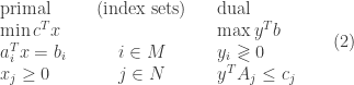
Equivalently, we can express it in a more familiar way

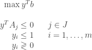
For canonical form ( ), we have

Property: Dual of dual is the primal. This is clear by observing that we may express the dual problem in (1) as

Taking the dual of (5) according to the definition from (1) yields the primal. Since the standard/canonical form primal-dual formulations are special cases of the general form, same property holds for (3) and (4). For the rest of the section we work mainly with the standard form.
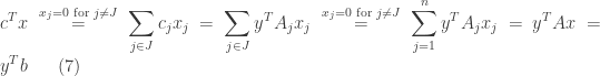
Property: Weak duality. The weak duality of LP problem is that, for any feasible solutions  to the primal and dual LP problems, the following holds

The first inequality is obtained by multiplying  on both sides of
  and the second by multiplying
  on both sides of
  .
.
Property: Strong duality. It turns out that the equalities hold for (6) when both are optimal solutions for the respective primal and dual LP problems. This is called the strong duality. To show this we will need Farka’s lemma based on the separating hyperplane theorem, which says that given two convex sets  that do not intersect trivially (the intersection does not contain any volume), there exists a hyperplane such that no two points
  lie in the same open halfspace created by the hyperplane. The separating hyperplane theorem, although intuitively true, is not trivial to prove; for more details see Convex Analysis, R. Tyrrell Rockafellar, pages 95-97. The variant of Farka’s lemma that we use is the following.
Theorem 1 (Farka’s lemma) Let  and
and  . Exactly one of the following holds:
- (a)
 such that
- (b)
 such that
  and
and  .
.
Proof. We need to show that a, b cannot be true at the same time and a  b. Note that
  . Also, the equations can be interpreted as “
 is a linear combination of the columns
  of
of  with coefficients
  :
:  ”.
”.
(a, b are mutually exclusive). The two conditions cannot hold at the same time, otherwise we have  by (a), which means that
  and
and  must have the same sign.
( ). We are now left to show that if the first condition fails, the second must be true. Note that we may view the columns of as
 -vectors in
  . Then
  for all
  is simply a cone
  of these -vectors which is convex and contains the zero vector. By assumption
  , the vector , which is simply a point in and thus convex, in not contained in . Moreover, if we take the ray from origin in the direction of , this is again convex and does not intersect non trivially. Thus, there exists a hyperplane that separates and . Clearly the hyperplane must pass through origin and we can pick its normal
  such that . For this , we have
  for each column
  of .
of .

We are now ready to prove the strong duality theorem. Assume that  is an optimal solution to the dual. Note that we may express the dual as
  . Let
. Let  be the set of (column) indices such that
  for
for  . That is, is the set of indices that are active. The set is not empty, otherwise is an interior point in the corresponding polytope representation of the feasible set. We see that there cannot be a vector
  , such that
  and
and  for , otherwise
  can be a better feasible solution for small
  since
since  and a small perturbation of will not violate the
 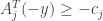 constraints. By Farka’s lemma, the other alternative must hold: For the set of ‘s with , there exists a set of ‘s such that
  and
and 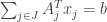 . If we let
  for
for  , we have
  , making
  a feasible solution to the primal problem. We then have
The strong duality theorem can be proved similarly for other primal-dual formulations. An immediate consequence of the strong duality property is that when the primal problem has an optimal, then the dual must also have an optimal and cannot be unbounded or infeasible. Same holds for dual-primal relationship. From the weak duality, we know that it is not possible for both primal and dual to be unbounded (having unbounded optimal cost). For the same reason, if primal/dual is unbounded, then the corresponding dual/primal must be infeasible. It is also possible that both primal and dual are infeasible. Examples can be found in the book.
Property: Complementary slackness. Another direct consequence of the strong duality property is complementary slackness. From (6) we observe that the following holds

with equality iff are optimal by the strong duality property. Complementary slackness holds for other primal-dual formulations as well, as a direct consequence of strong duality. Again, complementary slackness holds for other primal-dual formulations.
1.2. The primal dual algorithm
What can we do with duality? It turns out that there is quite a bit. We know that simplex algorithm may potential do an exponential number of pivoting. However, with primal dual algorithm, some problems can be solved in time polynomial in the size of the input. First, we will go through the basic procedure of carrying out the primal dual algorithm. To begin, we start with standard LP and its dual. First let us recall the primal dual formulation from last subsection

Note that we added  since this is always possible simply by flipping signs of some equations in . Now recall the complementary slackness condition, which says that for optimal , we always have

Since holds, second equality always holds for any feasible . Now assume that we have a feasible solution for the dual (D) (see the book for a simple way to get this), we let the set of indices denote those ‘s such that  ; for , can take any value. If we can get an that satisfies

Then the pair must be optimal by complementary slackness. Note that the set of ‘s in the first equality has since the rest are zeros. Of course, the set defined in above equation may be empty. This is where the primal dual algorithm comes in: We create an augmented primal, called restricted primal (RP), as follows:

The above restricted primal is feasible simply because we may let all and  to get a feasible solution. The cost is bounded below since it is non negative. If the (RP) above has an optimal solution with cost
  , then we found an optimal solution for P. But as we said, this cannot be guaranteed. Let us see what happens if the optimal solution does not have optimal cost . For this we move to the dual restricted primal (DRP), defined as the dual to (8), following the formula in (1):
Since it is the dual of (DP), which has an optimal solution, it has an optimal solution  . This solution satisfies
  and
and  . This suggest that for a feasible for (D),
  with may be a better solution than . Clearly, we cannot have
  for all
  ; otherwise we can make
  arbitrarily large (if this happens, then (P) is infeasible since (D) is unbounded). We are now left with the case that
  for some . On the other hand, recall that for , we have that
  . As we make
  larger, eventually for at least one more ,
  will be exactly
  . Thus, we have obtained a new feasible solution
  of (D) for which one or more will move to the set . At this point, we either get an optimal
  or we loop back to get another (RP) and then (DRP). Since every time at least one more is added, the process must end. This is the gist of the primal dual algorithm.
